
Suppose you get a $1,000 payment. How much do you spend? Before answering, we’d want to know a few things: Is this a one-time payment? The first of many? Can you borrow? Do you already have savings?
This year’s Nobel Prize in economics went to Robert Hall and Michael Woodford for providing the theory to make these questions concrete, the empirical work to test the theories, and an explanation of how both optimal and realistic policy differ depending on the answers.
When co-authors win the Nobel Prize, as in 2024, it’s pretty simple to see why they’re paired together. It makes a lot of sense.
This one takes a little more squinting. Woodford is a perennial favorite to win, and Hall is one of the great economists of all time, but he’s less often mentioned in Nobel discussions.
The Nobel Committee found a way to tie them together for “microeconomic foundations of macroeconomic stabilization”—how households’ and firms’ decisions inform policies to smooth the economy’s ups and downs. I’d say it’s “microeconomic foundations of macroeconomics,” or how those individual decisions shape the broader economy. But my guess is that this doesn’t sound important enough, so they wanted a “why does this matter?” hook. They went with “stabilization,” which immediately connects to policy.
This is a great macroeconomics prize. It’s partially a New Keynesian prize. New Keynesian economics describes how slow adjustments in prices and wages can give policy a role in stabilizing the economy. Woodford is basically synonymous with it, although Hall is less often described that way. As we’ll see, Hall’s equations and empirical approach became an essential part of the New Keynesian model.
I’ll go through some of Hall’s contributions: those directly connected to the prize, but also some the committee left out that I think are equally important and interesting. Then I’ll talk about how those contributions laid the foundation for Woodford’s work, which has been central to macroeconomics for more than 20 years.
Spending Tomorrow’s News Today
Going back to the $1,000 question, every question I asked is really getting at the same point: What does the payment tell you about your future income? A household that can borrow and save can spread that windfall, if it’s one-time, over many years. A temporary payment is really a small change in wealth. News that your income is permanently higher is a very different situation. It could generate a large change in your wealth.
That distinction between temporary and permanent income is what killed the old Keynesian consumption function, which tied spending to current income. Milton Friedman won his Nobel Prize partly for this—for his permanent income hypothesis, which ties spending to expected long-term income. One of Hall’s contributions was to make it precise and check it against the data. Hall is squarely in the Chicago price theory tradition, which uses prices and incentives to explain behavior, with this connection between individual decisions and the broader economy.
The hard part, empirically, is that expectations matter in the other direction, too. Suppose you learn today that you’re going to lose your job in six months. You may cut spending now, while your paycheck hasn’t changed. When you end up losing the job, the income drop may not be very large, and your spending may barely move.
By the late 1970s, economists had been writing down this sort of problem with rational expectations—the assumption that people use available information to make forecasts without systematic errors. A household that cares about consumption in every period chooses a path so that spending an extra dollar today and saving it to spend what it generates tomorrow offer the same expected benefit. That condition is the stochastic Euler equation—a rule for balancing consumption over time under uncertainty—which economics education drills into you.
In English, the left side is about what an extra dollar of consumption is worth today—the marginal utility of consumption. The right side is what that dollar is expected to be worth if you save it, earn interest at rate r, and spend it next period, discounted by beta, which reflects your impatience. At the optimum, the two are equal.
This is just the equimarginal principle: At the margin, equalize costs and benefits. What makes it slightly different, slightly macroeconomic, is that we have time—and, therefore, expectations.
You Can’t Read Minds, but You Can Test Them
A version of the stochastic Euler equation falls out of every modern macro model. Is it true? Does it show up in the data? Hall’s 1978 paper, “Stochastic Implications of the Life Cycle-Permanent Income Hypothesis,” turned this theory into something you could check.
The hard part is that you can’t observe what a household expects about future income. That expectation operator—the part of the equation above that represents those expectations—is tricky. Hall’s insight was that you don’t need to know expectations. Under his benchmark assumptions, consumption follows a random walk: Its changes reflect news, rather than information households already have. The basic idea is that anything households already know is in today’s spending, just as what the market believes about future earnings is in today’s stock price.
Today’s consumption is a very good predictor of tomorrow’s consumption. Nothing else households already know should improve that prediction. The question is whether other known information, like last year’s income, improves the forecast. If the theory holds, those extra variables shouldn’t add any predictive power.
The evidence was mixed, rather than a clear victory for this version of the permanent income hypothesis. Past income added little once the statistical analysis accounted for consumption, but stock prices were the exception. So we didn’t have a clear vindication or rebuttal of the model.
What Hall did show was how to turn a theory about unobservable expectations into a test using observable data. That’s a powerful connection from theory to data.
Interest Rates, Uninterested Consumers
Going back to the Euler equation, Hall’s 1978 paper really focuses on that expectations operator. But that’s not the only thing on the right-hand side. We can also ask whether there’s anything else we can pin down, like beta, the personal discount factor that reflects how much someone values future consumption relative to consumption today.
We can also ask about the interest rate. If monetary policy works by moving that price—the price between consumption today and consumption tomorrow—we can estimate the size of that response. A higher expected real return, meaning a return adjusted for inflation, makes postponing consumption more attractive. The elasticity of intertemporal substitution measures how strongly households respond by shifting consumption across time.
Hall’s 1988 paper on intertemporal substitution goes after that response. Now let’s look at the very fancy plots you’d find in a 1980s economics paper.
Each point is a five-year average of the real return from Treasury bills, plotted against the growth rate of consumption. A strong response to the interest rate would show up as an upward-sloping set of dots. That’s not what we see. To be clear, this is just a descriptive illustration. It’s not how Hall actually estimates the elasticity.
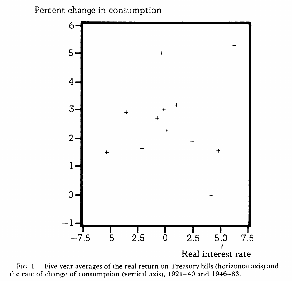
This plot of prices (interest rates) and quantities (consumption) has the usual identification problem: We only observe the price and quantity where supply and demand meet, and either could move as supply or demand shifts. We instead want to see how consumption changes when r moves for reasons unrelated to the other forces affecting consumption.
Hall’s solution is the usual one for estimating a demand curve. You can’t just run a statistical analysis relating price to quantity. You need to find variation in the price that has nothing to do with the shocks to whatever you’re trying to explain.
This is where the theory helps, where the Euler equation matters. It says households act on the expected real return. Variables known before the consumption change that help predict that return, like earlier interest rates or earlier inflation, are information households could have used. They aren’t shocks or surprises to consumption. You can use those as instruments—variables that help isolate the relevant variation in returns—and ask whether the part of the expected return they predict lines up with consumption growth.
The measure of price needs care, too. The return that matters is the expected real return after taxes, not the realized one, so you’ve got to be careful with that. Hall has spent much of his career being precise about these things. This isn’t a post about the details of measuring post-tax returns. The important thing is that Hall filled in the details, moving from the model to its testable implications.
So did the interest rate matter? Not really.
The elasticity could be zero, and it’s probably no higher than 0.2—a relatively weak response. But this was a start at measuring it, not the tightest estimate ever. A 1988 paper with aggregate data—figures for the economy as a whole—isn’t the end of the empirical discussion. As with many prizes, this one is about launching a whole research program.
Hall’s low elasticity leaves a puzzle. If households barely shift consumption across time when the real interest rate moves, how does a rate cut raise spending at all?
But Wait, There’s More Hall
If you go to Hall’s Google Scholar page, you’ll see that these consumption papers are only his second- and sixth-most-cited papers. He has done so much, including developing a popular optimization algorithm—a method for finding the best solution to a mathematical problem. As Tyler Cowen rightly put it, “Every Bob Hall paper is interesting!”
Let me focus on two that I think are core price theory.
Even if you buy the machine, you pay its rental price every period in the form of income you give up, because you could be renting it to someone else. Owning does not make its services free. Hall and Dale Jorgenson’s 1967 paper, which they wrote while Hall was a graduate student, built an empirical investment model on that idea.
The sticker price is not the cost of using the machine for a year. The firm ties up money, the machine depreciates—loses value through use and aging—and its resale price may change. The cost of using capital is roughly the price of the capital good multiplied by the sum of the interest rate and the depreciation rate, less expected capital gains.
The firm compares what the machine adds to output with that user cost, and the paper estimates how much investment responds and when. It’s the household problem again, with the real interest rate as the price of time.
The other paper is Hall’s 1988 article in the Journal of Political Economy on price and marginal cost. The Nobel Committee cites it in the scientific background, but I’m pretty sure that reference is a typo.
What does producing one more unit actually cost? That’s marginal cost. Firms don’t report it, but we can observe how their inputs change when they produce more. The problem is that this tests competition and constant returns—the assumption that doubling inputs doubles output—together. We’re always doing a joint test, but that’s a topic for another day.
That is classic Hall: Let’s take something we don’t directly observe and work out how to test it using choices we do observe.
The markup paper, which examines the gap between price and marginal cost, also sets up Woodford’s work nicely, with its sticky prices—prices that adjust slowly—and markups. That holds even though the Nobel Committee cites it in a very confusing way.
A Model With People in It
Suppose the central bank wants to know what happens if it raises the interest rate by 1 percentage point. Instead of the old approach of estimating how inflation moves with unemployment, you want to start with a microfounded approach—as the Nobel Prize points out—based on how households and firms make decisions. Then you can make causal claims. You need to know what causes what.
The problem with correlations is that people’s behavior changes depending on the policies they live under. This is the classic Lucas critique, named for economist Robert Lucas. In the 1960s, higher inflation came with lower unemployment, so policymakers tried to exploit that relationship. People came to expect inflation. The 1970s gave us high inflation and high unemployment together.
Woodford’s contribution was to tie the pieces into one causal chain. The Nobel Committee’s scientific background lays it out, following his book “Interest and Prices.”
The benchmark New Keynesian model has just three equations.
The first is Hall’s Euler equation with some bells and whistles. Add the “natural rate”—the interest rate consistent with stable inflation and the economy operating at its potential—drawing on economist Knut Wicksell, and you basically have it.
The second equation comes from firms. A restaurant that reprints its menu once a year—a simple assumption to capture sticky prices—has to guess at costs and demand for the whole year its prices will be in use. Firms that can’t change prices every period face the same problem, so their pricing looks forward.
Then you close the model with an interest rate rule. The central bank sets its interest rate in response to inflation and the output gap—the difference between actual output and the economy’s potential—as in a Taylor rule, named for economist John Taylor. That closes the loop.
So you have these three equations feeding back into each other. Every link is a choice someone makes. Everyone is looking ahead, and when you change the rules, people change what they expect. That feeds into their behavior. This allows us to work through responses without assuming people will behave as they did under the old policy. That’s the benefit of microfoundations.
Does this particular microfounded macro model match the data? Yes and no.
The Model Gets Two Out of Three
Everyone knows the book, “Interest and Prices,” but the easiest way into the project is Woodford’s 1997 paper with Julio Rotemberg. They built a quantitative model from households and firms making choices to achieve their goals and used it to evaluate monetary policy rules. The first question is whether the model can reproduce what happens after an unexpected Federal Reserve rate increase.
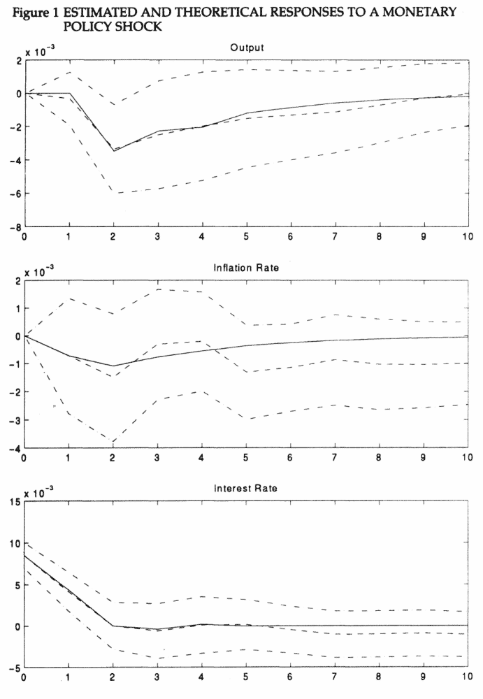
It’s a weird way of showing it, but the bottom panel shows the shock—the unexpected rate increase.
The interest rate rises, then returns to normal within a couple of quarters. In the top panel, output falls with a delay and recovers gradually. The model’s solid line closely follows the middle line representing the estimated response in both panels.
The middle panel is harder. The estimated inflation response stays negative longer than the model’s does. Matching how long inflation stays low is the weak spot.
They then asked what different rules would do. In their model, a better rule stabilizes inflation more and output less than the policy they estimated the Fed followed.
Zero Interest, Great Expectations
The other paper I want to cover is Gauti Eggertsson and Woodford (2003), on the zero lower bound—the point at which interest rates reach zero. Yes, 2003. It responded to Japan’s near-zero interest rates, weak growth, and falling prices, but proved much more relevant after 2008.
What can a central bank do when its usual tool—cutting the rate—is gone?
We can think through this with the New Keynesian model. The zero bound is a price floor for the nominal interest rate—the rate before adjusting for inflation—but we have all these other parts of the equations. We have the distinction between real and nominal rates. We also have expectations about future policy, and those turn out to be the key.
The central bank can promise to keep rates low even after the zero-bound constraint no longer limits its choices. That changes the income and returns households expect, so they can spend more today.
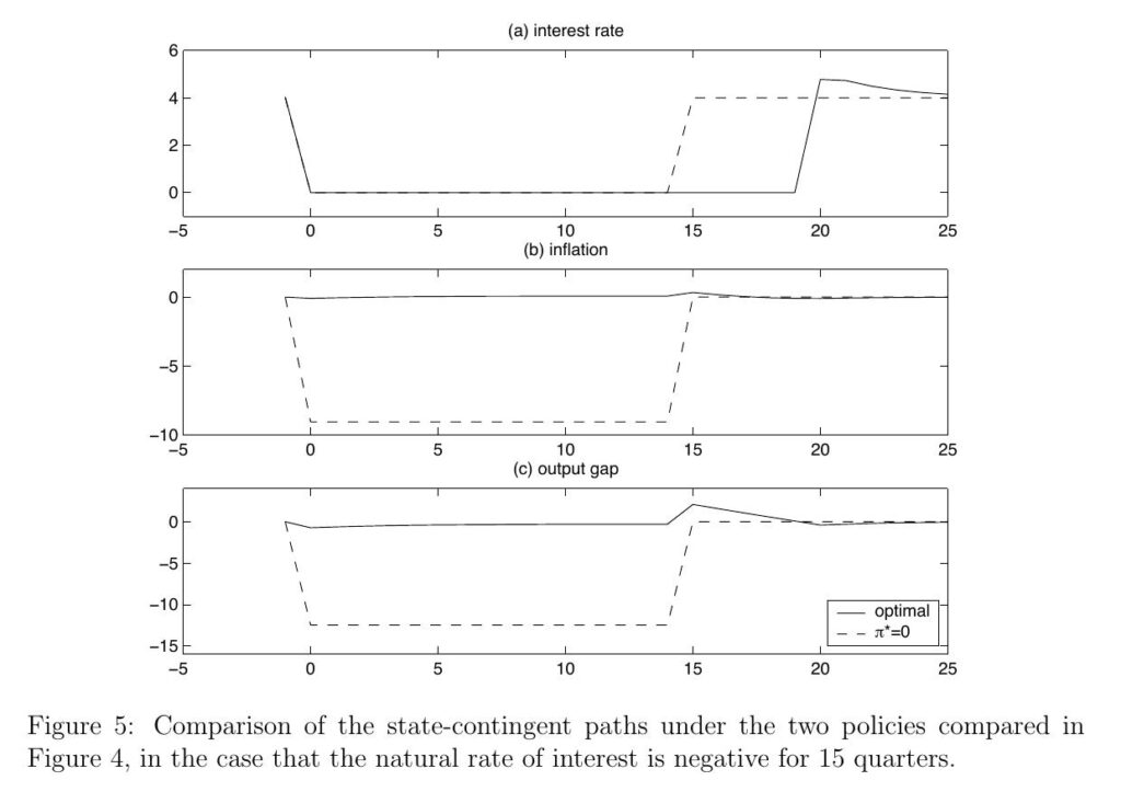
We can’t run experiments on the Fed. We only see the policies central banks actually chose, never what would have happened under the alternatives. A model that gets household and firm behavior right lets us change the rule and follow the responses through spending, prices, and expectations.
Overall, Woodford’s work and the New Keynesian model provide the benchmark for these types of thought experiments.
This is a long post already, so I’m not going to go through my gripes with the New Keynesian model. I’d simply refer people to John Cochrane on the issues with how the model determines inflation at all.
The model has no money. See Ricardo Lagos on whether we can safely ignore money, and Joshua Hendrickson on whether we’re measuring it right.
That is great price theory in the Friedman tradition, and I’m especially happy with Hall’s half of this prize. The model is wrong in plenty of ways. But a model like this gives us something concrete to argue about.
For more on prizes in this series, read last year’s post on Joel Mokyr, Philippe Aghion, and Peter Howitt, as well as earlier posts on the 2024 prize and the 2023 prize.